Performing Viterbi Decoding

The Viterbi decoder itself is the primary focus of this tutorial. Perhaps the single most important concept to aid in understanding the Viterbi algorithm is the trellis diagram. The figure below shows the trellis diagram for our example rate 1/2 K = 3 convolutional encoder, for a 15-bit message:

The four possible states of the encoder are depicted as four rows of horizontal dots. There is one column of four dots for the initial state of the encoder and one for each time instant during the message. For a 15-bit message with two encoder memory flushing bits, there are 17 time instants in addition to t = 0, which represents the initial condition of the encoder. The solid lines connecting dots in the diagram represent state transitions when the input bit is a one. The dotted lines represent state transitions when the input bit is a zero. Notice the correspondence between the arrows in the trellis diagram and the state transition table discussed above. Also notice that since the initial condition of the encoder is State 00₂, and the two memory flushing bits are zeroes, the arrows start out at State 00₂ and end up at the same state.

The following diagram shows the states of the trellis that are actually reached during the encoding of our example 15-bit message:

The encoder input bits and output symbols are shown at the bottom of the diagram. Notice the correspondence between the encoder output symbols and the output table discussed above. Let's look at that in more detail, using the expanded version of the transition between one time instant to the next shown below:

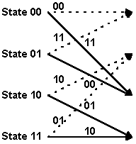
The two-bit numbers labeling the lines are the corresponding convolutional encoder channel symbol outputs. Remember that dotted lines represent cases where the encoder input is a zero, and solid lines represent cases where the encoder input is a one. (In the figure above, the two-bit binary numbers labeling dotted lines are on the left, and the two-bit binary numbers labeling solid lines are on the right.)

OK, now let's start looking at how the Viterbi decoding algorithm actually works. For our example, we're going to use hard-decision symbol inputs to keep things simple. (The example source code uses soft-decision inputs to achieve better performance.) Suppose we receive the above encoded message with a couple of bit errors:

Each time we receive a pair of channel symbols, we're going to compute a metric to measure the "distance" between what we received and all of the possible channel symbol pairs we could have received. Going from t = 0 to t = 1, there are only two possible channel symbol pairs we could have received: 00₂, and 11₂. That's because we know the convolutional encoder was initialized to the all-zeroes state, and given one input bit = one or zero, there are only two states we could transition to and two possible outputs of the encoder. These possible outputs of the encoder are 00 ₂ and 11₂.

The metric we're going to use for now is the Hamming distance between the received channel symbol pair and the possible channel symbol pairs. The Hamming distance is computed by simply counting how many bits are different between the received channel symbol pair and the possible channel symbol pairs. The results can only be zero, one, or two. The Hamming distance (or other metric) values we compute at each time instant for the paths between the states at the previous time instant and the states at the current time instant are called branch metrics. For the first time instant, we're going to save these results as "accumulated error metric" values, associated with states. For the second time instant on, the accumulated error metrics will be computed by adding the previous accumulated error metrics to the current branch metrics.

At t = 1, we received 00_2. The only possible channel symbol pairs we could have received are 00₂ and 11₂. The Hamming distance between 00₂ and 00₂ is zero. The Hamming distance between 00₂ and 11₂ is two. Therefore, the branch metric value for the branch from State 00₂ to State 00₂ is zero, and for the branch from State 00₂ to State 10₂ it's two. Since the previous accumulated error metric values are equal to zero, the accumulated metric values for State 00₂ and for State 10₂ are equal to the branch metric values. The accumulated error metric values for the other two states are undefined. The figure below illustrates the results at t = 1:

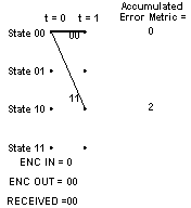
Note that the solid lines between states at t = 1 and the state at t = 0 illustrate the predecessor-successor relationship between the states at t = 1 and the state at t = 0 respectively. This information is shown graphically in the figure, but is stored numerically in the actual implementation. To be more specific, or maybe clear is a better word, at each time instant t, we will store the number of the predecessor state that led to each of the current states at t.

Now let's look what happens at t = 2. We received a 11₂ channel symbol pair. The possible channel symbol pairs we could have received in going from t = 1 to t = 2 are 00₂ going from State 00₂ to State 00₂, 11₂ going from State 00₂ to State 10₂, 10₂ going from State 10₂ to State 01 ₂, and 01₂ going from State 10₂ to State 11 ₂. The Hamming distance between 00₂ and 11₂ is two, between 11₂ and 11₂ is zero, and between 10 ₂ or 01₂ and 11₂ is one. We add these branch metric values to the previous accumulated error metric values associated with each state that we came from to get to the current states. At t = 1, we could only be at State 00₂ or State 10₂. The accumulated error metric values associated with those states were 0 and 2 respectively. The figure below shows the calculation of the accumulated error metric associated with each state, at t = 2.

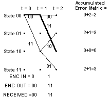
That's all the computation for t = 2. What we carry forward to t = 3 will be the accumulated error metrics for each state, and the predecessor states for each of the four states at t = 2, corresponding to the state relationships shown by the solid lines in the illustration of the trellis.

Now look at the figure for t = 3. Things get a bit more complicated here, since there are now two different ways that we could get from each of the four states that were valid at t = 2 to the four states that are valid at t = 3. So how do we handle that? The answer is, we compare the accumulated error metrics associated with each branch, and discard the larger one of each pair of branches leading into a given state. If the members of a pair of accumulated error metrics going into a particular state are equal, we just save that value. The other thing that's affected is the predecessor-successor history we're keeping. For each state, the predecessor that survives is the one with the lower branch metric. If the two accumulated error metrics are equal, some people use a fair coin toss to choose the surviving predecessor state. Others simply pick one of them consistently, i.e. the upper branch or the lower branch. It probably doesn't matter which method you use. The operation of adding the previous accumulated error metrics to the new branch metrics, comparing the results, and selecting the smaller (smallest) accumulated error metric to be retained for the next time instant is called the add-compare-select operation. The figure below shows the results of processing t = 3:

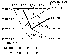
Note that the third channel symbol pair we received had a one-symbol error. The smallest accumulated error metric is a one, and there are two of these.

Let's see what happens now at t = 4. The processing is the same as it was for t = 3. The results are shown in the figure:

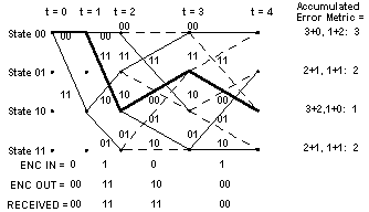
Notice that at t = 4, the path through the trellis of the actual transmitted message, shown in bold, is again associated with the smallest accumulated error metric. Let's look at t = 5:

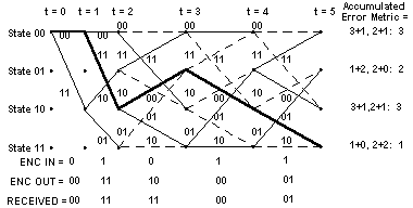
At t = 5, the path through the trellis corresponding to the actual message, shown in bold, is still associated with the smallest accumulated error metric. This is the thing that the Viterbi decoder exploits to recover the original message.

Perhaps you're getting tired of stepping through the trellis. I know I am. Let's skip to the end.

At t = 17, the trellis looks like this, with the clutter of the intermediate state history removed:

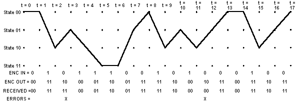
The decoding process begins with building the accumulated error metric for some number of received channel symbol pairs, and the history of what states preceded the states at each time instant t with the smallest accumulated error metric. Once this information is built up, the Viterbi decoder is ready to recreate the sequence of bits that were input to the convolutional encoder when the message was encoded for transmission. This is accomplished by the following steps:

• First, select the state having the smallest accumulated error metric and save the state number of that state.
• Iteratively perform the following step until the beginning of the trellis is reached: Working backward through the state history table, for the selected state, select a new state which is listed in the state history table as being the predecessor to that state. Save the state number of each selected state. This step is called traceback.
• Now work forward through the list of selected states saved in the previous steps. Look up what input bit corresponds to a transition from each predecessor state to its successor state. That is the bit that must have been encoded by the convolutional encoder.

It is interesting to note that for this hard-decision-input Viterbi decoder example, the smallest accumulated error metric in the final state indicates how many channel symbol errors occurred.

The following state history table shows the surviving predecessor states for each state at each time t:
 

The following table shows the states selected when tracing the path back through the survivor state table shown above:
 

Using a table that maps state transitions to the inputs that caused them, we can now recreate the original message. Here is what this table looks like for our example rate 1/2 K = 3 convolutional code:
 

Note: In the above table, x denotes an impossible transition from one state to another state.

So now we have all the tools required to recreate the original message from the message we received:
 

The two flushing bits are discarded.

Here's an insight into how the traceback algorithm eventually finds its way onto the right path even if it started out choosing the wrong initial state. This could happen if more than one state had the smallest accumulated error metric, for example. I'll use the figure for the trellis at t = 3 again to illustrate this point:

See how at t = 3, both States 01₂ and 11₂ had an accumulated error metric of 1. The correct path goes to State 01₂ -notice that the bold line showing the actual message path goes into this state. But suppose we choose State 11₂ to start our traceback. The predecessor state for State 11₂ , which is State 10₂ , is the same as the predecessor state for State 01₂! This is because at t = 2, State 10₂ had the smallest accumulated error metric. So after a false start, we are almost immediately back on the correct path.

For the example 15-bit message, we built the trellis up for the entire message before starting traceback. For longer messages, or continuous data, this is neither practical or desirable, due to memory constraints and decoder delay. Research has shown that a traceback depth of K x 5 is sufficient for Viterbi decoding with the type of codes we have been discussing. Any deeper traceback increases decoding delay and decoder memory requirements, while not significantly improving the performance of the decoder. The exception is punctured codes, which I'll describe later. They require deeper traceback to reach their final performance limits.

To implement a Viterbi decoder in software, the first step is to build some data structures around which the decoder algorithm will be implemented. These data structures are best implemented as arrays. The primary six arrays that we need for the Viterbi decoder are as follows:

• A copy of the convolutional encoder next state table, the state transition table of the encoder. The dimensions of this table (rows x columns) are 2^{(K - 1)} x 2^k. This array needs to be initialized before starting the decoding process.
• A copy of the convolutional encoder output table. The dimensions of this table are 2^{(K - 1)} x 2^k. This array needs to be initialized before starting the decoding process.
• An array (table) showing for each convolutional encoder current state and next state, what input value (0 or 1) would produce the next state, given the current state. We'll call this array the input table. Its dimensions are 2^{(K - 1)} x 2^{(K - 1)}. This array needs to be initialized before starting the decoding process.
• An array to store state predecessor history for each encoder state for up to K x 5 + 1 received channel symbol pairs. We'll call this table the state history table. The dimensions of this array are 2 ^{(K - 1)} x (K x 5 + 1). This array does not need to be initialized before starting the decoding process.
• An array to store the accumulated error metrics for each state computed using the add-compare-select operation. This array will be called the accumulated error metric array. The dimensions of this array are 2 ^{(K - 1)} x 2. This array does not need to be initialized before starting the decoding process.
• An array to store a list of states determined during traceback (term to be explained below). It is called the state sequence array. The dimensions of this array are (K x 5) + 1. This array does not need to be initialized before starting the decoding process.

where a one indicates that a channel symbol is to be transmitted, and a zero indicates that a channel symbol is to be deleted. To see how this make the rate be 3/4, think of each column of the above table as corresponding to a bit input to the encoder, and each one in the table as corresponding to an output channel symbol. There are three columns in the table, and four ones. You can even create a rate 2/3 code using a rate 1/2 encoder with the following puncturing pattern:
 

which has two columns and three ones.

To decode a punctured code, one must substitute null symbols for the deleted symbols at the input to the Viterbi decoder. Null symbols can be symbols quantized to levels corresponding to weak ones or weak zeroes, or better, can be special flag symbols that when processed by the ACS circuits in the decoder, result in no change to the accumulated error metric from the previous state.

Of course, n does not have to be equal to two. For example, a rate 1/3, K = 3, (7, 7, 5) code can be encoded using the encoder shown below:

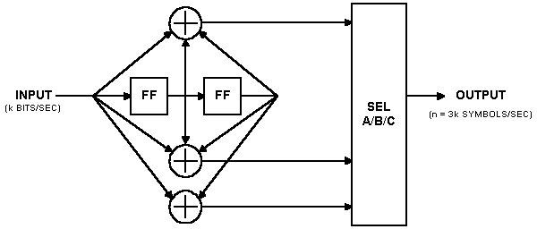
This encoder has three modulo-two adders, so for each input bit, it can produce three channel symbol outputs. Of course, with suitable puncturing patterns, you can create higher-rate codes using this encoder as well.

I don't have good data to share with you right now about the traceback depth requirements for Viterbi decoders for punctured codes. I have been told that instead of K x 5, depths of K x 7, K x 9, or even more are required to reach the point of diminishing returns. This would be a good topic around which to design some experiments using a modified version of the example simulation code I provide.

Click on one of the links below to go to the beginning of that section:

 Introduction
 Description of the Algorithms  (Part 1)
 Simulation Source Code Examples
 Example Simulation Results
 Bibliography
 About Spectrum Applications...