
The steps involved in simulating a communication channel using convolutional encoding and Viterbi decoding are as follows:
Generating the data to be transmitted through the channel can be accomplished quite simply by using a random number generator. One that produces a uniform distribution of numbers on the interval 0 to a maximum value is provided in C: rand (). Using this function, we can say that any value less than half of the maximum value is a zero; any value greater than or equal to half of the maximum value is a one.
Convolutionally Encoding the Data
Convolutionally encoding the data is accomplished using a shift register and associated combinatorial logic that performs modulo-two addition. (A shift register is merely a chain of flip-flops wherein the output of the nth flip-flop is tied to the input of the (n+1)th flip-flop. Every time the active edge of the clock occurs, the input to the flip-flop is clocked through to the output, and thus the data are shifted over one stage.) The combinatorial logic is often in the form of cascaded exclusive-or gates. As a reminder, exclusive-or gates are two-input, one-output gates often represented by the logic symbol shown below,
that implement the following truth-table:
|
|
|
(A xor B) |
|
|
|
|
|
|
|
|
|
|
|
|
|
|
|
|
The exclusive-or gate performs modulo-two addition of its inputs. When you cascade q two-input exclusive-or gates, with the output of the first one feeding one of the inputs of the second one, the output of the second one feeding one of the inputs of the third one, etc., the output of the last one in the chain is the modulo-two sum of the q + 1 inputs.
Another way to illustrate the modulo-two adder, and the way that is most commonly used in textbooks, is as a circle with a + symbol inside, thus:
![]()
Now that we have the two basic components of the convolutional encoder (flip-flops comprising the shift register and exclusive-or gates comprising the associated modulo-two adders) defined, let's look at a picture of a convolutional encoder for a rate 1/2, K = 3, m = 2 code:
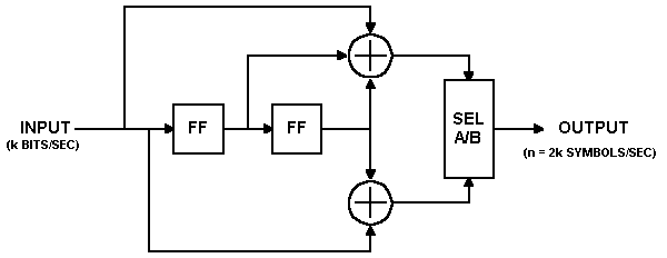
In this encoder, data bits are provided at a rate of k bits per second. Channel symbols are output at a rate of n = 2k symbols per second. The input bit is stable during the encoder cycle. The encoder cycle starts when an input clock edge occurs. When the input clock edge occurs, the output of the left-hand flip-flop is clocked into the right-hand flip-flop, the previous input bit is clocked into the left-hand flip-flop, and a new input bit becomes available. Then the outputs of the upper and lower modulo-two adders become stable. The output selector (SEL A/B block) cycles through two states-in the first state, it selects and outputs the output of the upper modulo-two adder; in the second state, it selects and outputs the output of the lower modulo-two adder.
The encoder shown above encodes the K = 3, (7, 5) convolutional code. The octal numbers 7 and 5 represent the code generator polynomials, which when read in binary (1112 and 1012) correspond to the shift register connections to the upper and lower modulo-two adders, respectively. This code has been determined to be the "best" code for rate 1/2, K = 3. It is the code I will use for the remaining discussion and examples, for reasons that will become readily apparent when we get into the Viterbi decoder algorithm.
Let's look at an example input data stream, and the corresponding output data stream:
Let the input sequence be 0101110010100012.
Assume that the outputs of both of the flip-flops in the shift register are initially cleared, i.e. their outputs are zeroes. The first clock cycle makes the first input bit, a zero, available to the encoder. The flip-flop outputs are both zeroes. The inputs to the modulo-two adders are all zeroes, so the output of the encoder is 002.
The second clock cycle makes the second input bit available to the encoder. The left-hand flip-flop clocks in the previous bit, which was a zero, and the right-hand flip-flop clocks in the zero output by the left-hand flip-flop. The inputs to the top modulo-two adder are 1002, so the output is a one. The inputs to the bottom modulo-two adder are 102, so the output is also a one. So the encoder outputs 112 for the channel symbols.
The third clock cycle makes the third input bit, a zero, available to the encoder. The left-hand flip-flop clocks in the previous bit, which was a one, and the right-hand flip-flop clocks in the zero from two bit-times ago. The inputs to the top modulo-two adder are 0102, so the output is a one. The inputs to the bottom modulo-two adder are 002, so the output is zero. So the encoder outputs 102 for the channel symbols.
And so on. The timing diagram shown below illustrates the process:
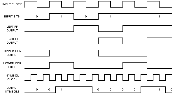
After all of the inputs have been presented to the encoder, the output sequence will be:
00 11 10 00 01 10 01 11 11 10 00 10 11 00 112.
Notice that I have paired the encoder outputs-the first bit in each pair is the output of the upper modulo-two adder; the second bit in each pair is the output of the lower modulo-two adder.
You can see from the structure of the rate 1/2 K = 3 convolutional encoder and from the example given above that each input bit has an effect on three successive pairs of output symbols. That is an extremely important point and that is what gives the convolutional code its error-correcting power. The reason why will become evident when we get into the Viterbi decoder algorithm.
Now if we are only going to send the 15 data bits given above, in order for the last bit to affect three pairs of output symbols, we need to output two more pairs of symbols. This is accomplished in our example encoder by clocking the convolutional encoder flip-flops two ( = m) more times, while holding the input at zero. This is called "flushing" the encoder, and results in two more pairs of output symbols. The final binary output of the encoder is thus 00 11 10 00 01 10 01 11 11 10 00 10 11 00 11 10 112. If we don't perform the flushing operation, the last m bits of the message have less error-correction capability than the first through (m - 1)th bits had. This is a pretty important thing to remember if you're going to use this FEC technique in a burst-mode environment. So's the step of clearing the shift register at the beginning of each burst. The encoder must start in a known state and end in a known state for the decoder to be able to reconstruct the input data sequence properly.
Now, let's look at the encoder from another perspective. You can think
of the encoder as a simple state machine. The example encoder has two bits
of memory, so there are four possible states. Let's give the left-hand
flip-flop a binary weight of 21, and the right-hand flip-flop
a binary weight of 20. Initially, the encoder is in the all-zeroes
state. If the first input bit is a zero, the encoder stays in the all zeroes
state at the next clock edge. But if the input bit is a one, the encoder
transitions to the 102 state at the next clock edge. Then, if
the next input bit is zero, the encoder transitions to the 012
state, otherwise, it transitions to the 112 state. The following
table gives the next state given the current state and the input, with
the states given in binary:
|
|
||
|
|
|
|
|
|
|
|
|
|
|
|
|
|
|
|
|
|
|
|
The above table is often called a state transition table. We'll refer
to it as the next state table. Now let us look at a table
that lists the channel output symbols, given the current state and the
input data, which we'll refer to as the output table:
|
|
||
|
|
|
|
|
|
|
|
|
|
|
|
|
|
|
|
|
|
|
|
You should now see that with these two tables, you can completely describe the behavior of the example rate 1/2, K = 3 convolutional encoder. Note that both of these tables have 2(K - 1) rows, and 2k columns, where K is the constraint length and k is the number of bits input to the encoder for each cycle. These two tables will come in handy when we start discussing the Viterbi decoder algorithm.
Mapping the Channel Symbols to Signal Levels
Mapping the one/zero output of the convolutional encoder onto an antipodal baseband signaling scheme is simply a matter of translating zeroes to +1s and ones to -1s. This can be accomplished by performing the operation y = 1 - 2x on each convolutional encoder output symbol.
Adding Noise to the Transmitted Symbols
Adding noise to the transmitted channel symbols produced by the convolutional encoder involves generating Gaussian random numbers, scaling the numbers according to the desired energy per symbol to noise density ratio, Es/N 0, and adding the scaled Gaussian random numbers to the channel symbol values.
For the uncoded channel, Es/N0 = Eb/N 0, since there is one channel symbol per bit. However, for the coded channel, Es/N0 = Eb/N0 + 10log10(k/n). For example, for rate 1/2 coding, E s/N0 = Eb/N0 + 10log10(1/2) = Eb/N0 - 3.01 dB. Similarly, for rate 2/3 coding, Es/N0 = Eb/N0 + 10log10 (2/3) = Eb/N0 - 1.76 dB.
The Gaussian random number generator is the only interesting part of this task. C only provides a uniform random number generator, rand(). In order to obtain Gaussian random numbers, we take advantage of relationships between uniform, Rayleigh, and Gaussian distributions:
Given a uniform random variable U, a Rayleigh random variable R can be obtained by:
![]()
where ![]() is the variance of the Rayleigh random variable, and given R and a second
uniform random variable V, two Gaussian random variables G and H can be
obtained by
is the variance of the Rayleigh random variable, and given R and a second
uniform random variable V, two Gaussian random variables G and H can be
obtained by
G = R cos V and H = R sin V.
In the AWGN channel, the signal is corrupted by additive noise, n(t),
which has the power spectrum No/2 watts/Hz. The variance ![]() of this noise is equal to
of this noise is equal to ![]() . If we set the energy per symbol Es equal to 1, then
. If we set the energy per symbol Es equal to 1, then ![]() . So
. So ![]() .
.
Quantizing the Received Channel Symbols
An ideal Viterbi decoder would work with infinite precision, or at least with floating-point numbers. In practical systems, we quantize the received channel symbols with one or a few bits of precision in order to reduce the complexity of the Viterbi decoder, not to mention the circuits that precede it. If the received channel symbols are quantized to one-bit precision (< 0V = 1, > 0V = 0), the result is called hard-decision data. If the received channel symbols are quantized with more than one bit of precision, the result is called soft-decision data. A Viterbi decoder with soft decision data inputs quantized to three or four bits of precision can perform about 2 dB better than one working with hard-decision inputs. The usual quantization precision is three bits. More bits provide little additional improvement.
The selection of the quantizing levels is an important design decision
because it can have a significant effect on the performance of the link.
The following is a very brief explanation of one way to set those levels.
Let's assume our received signal levels in the absence of noise are -1V
= 1, +1V = 0. With noise, our received signal has mean +/- 1 and standard
deviation ![]() . Let's use a uniform, three-bit quantizer having the input/output relationship
shown in the figure below, where D is a decision level that we will calculate
shortly:
. Let's use a uniform, three-bit quantizer having the input/output relationship
shown in the figure below, where D is a decision level that we will calculate
shortly:
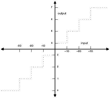
The decision level, D, can be calculated according to the formula ![]() , where Es/N0 is the energy per symbol to noise density
ratio. (The above figure was redrawn from Figure 2 of Advanced Hardware
Architecture's ANRS07-0795, "Soft Decision Thresholds and Effects on Viterbi
Performance". See the bibliography
for a link to their web pages.)
, where Es/N0 is the energy per symbol to noise density
ratio. (The above figure was redrawn from Figure 2 of Advanced Hardware
Architecture's ANRS07-0795, "Soft Decision Thresholds and Effects on Viterbi
Performance". See the bibliography
for a link to their web pages.)
Click here to proceed to the description of the Viterbi decoding algorithm itself...
Or click on one of the links below to go to the beginning of that section:
Introduction
Description of the Algorithms
(Part 2)
Simulation Source Code Examples
Example Simulation Results
Bibliography
About Spectrum Applications...